DirectXGraphics: Cubic Terrain Patches
Author: Jack Hoxley
Written: 10th May 2002
Contact: [Email]
Download: GR_Cubic.Zip (138kb)

Contents of this lesson
1. Introduction
2. The Cubic Equations

1. Introduction

Welcome to another extended DirectXGraphics article. This isn't going to be a tutorial as such, more of a covering-note for the downloadable source code.

I have a considerable interest in terrain modeling, and often read articles/white-papers on the subject. One area that crops up every so often is the use of quadratic/cubic/quartic/quintic patches to approximate an area of terrain. There are many advantages to this - the mathematical nature of the terrain makes it easy to implement LOD (Level Of Detail) algorithms, and it also provides nice results :-)

So, just for fun I decided to re-read several articles that I found and see if I could get it working in VB, and the fact that you're now reading this text shows that I managed to do it - and maybe you'd be interested in seeing how it all works!

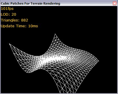
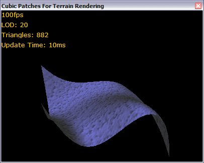
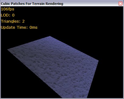
The following 6 pictures show (in wireframe and solid forms) what the results are, the LOD is scalar, so the higher it is the smoother the terrain (but the more triangles / slower it gets).

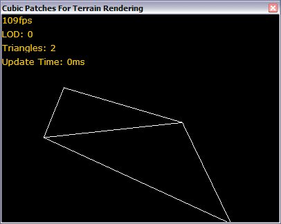
Above and below: The lowest (0) possible setting

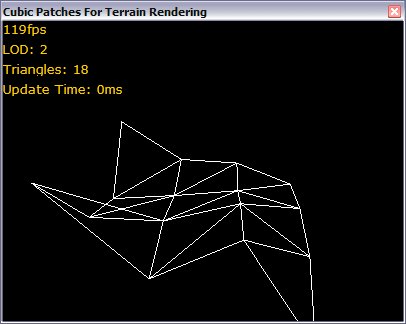
Above and Below: A low setting, but starting to look better!

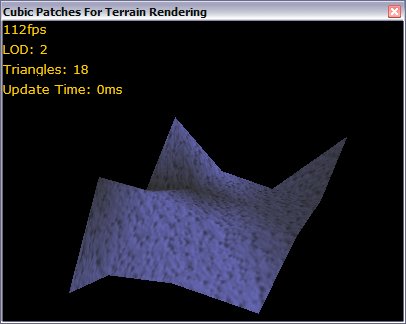
Above and Below: A high resolution render, note very smooth :)

2. The Cubic Equations

The equations used to generate these "patches" are quite simple if you're good at math's, but if you're not familiar with parametric equations you'll need to do some research before continuing (I don't have the time to teach/explain them properly!)

First we take the simple linear equation: 
(A+B)=1
where A is the distance from the start (0.0 to 1.0) and B is the distance from the end (0.0 to 1.0). This basically expands to:
A + t(B-A)
with a little work.

We can then extend this to be "to the power n" - 2 (Quadratic), 3 (Cubic), 4 (Quartic), 5 (Quintic). When we raise it to one of these powers we need to multiply out the brackets, which gives us the polynomial to power n. For example:

(A+B)² = A² + 2AB + B²
(A+B)³ = A³ + 3A²B + 3AB² + B³
(A+B)⁴ = A⁴ + 4A³B + 6A²B² + 4AB³ + B⁴
(A+B)⁵ = A⁵ + 5A⁴B + 10A²B³ + 5AB⁴ + B⁵

I'm going to focus on the cubic equation, but you can easily work out the other versions if you really want them...

if we take A and B to be the distances along the line, we need to express them as one parameter (so we can get an f(t) formatted function). using the linear equation above:
(A+B)³ = 1     'cube-root both sides
(A+B) = 1       'cube root of 1 is still 1
B = 1-A          'rearrange for B

if we now substitute this into the main cubic equation:

A³ + 3A²(1-A) + 3A(1-A)² + (1-A)³

don't simplify it yet, as all you'll do is prove that 1=1 or 0=0 :-)

to control our curve we're going to add a coefficient to each term of the equation and consider them to be "control points" - these are additional 3D points that will "guide" the curve accordingly. I will use lower case letters a, b, c, d (don't muddle these with A and B).

aA³ + b3A²(1-A) + c3A(1-A)² + d(1-A)³

as it stands, with parameter A being in the range 0<=A<=1, control point 'a' is the start of the line (A=0.0), 'd' is the end of the line (A=1.0) and points 'b' and 'c' are just used to guide the curve (the curve wont actually pass through these points).

We can now expand these into the final parametric equations:

X(A) = a_xA³ + b_x3A²(1-A) + c_x3A(1-A)² + d_x(1-A)³
Y(A) = a_yA³ + b_y3A²(1-A) + c_y3A(1-A)² + d_y(1-A)³
Z(A) = a_zA³ + b_z3A²(1-A) + c_z3A(1-A)² + d_z(1-A)³

^{These equations will work perfectly for drawing a line between 'a' and 'd' influenced by 'c' and 'd'}

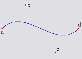
An example of a cubic spline

Okay, we now need to expand this to cover a 2D patch, where we pass in an x and y value, and we get the "height" at the given point (this is the equation used to generate the meshes shown above).

(A+B)³•(C+D)³=1

basically, we just multiply the two curves, and we'll get the desired result!

(A³ + 3A²B + 3AB² + B³)•(A³ + 3A²B + 3AB² + B³)

I'll just jump to the full parametric equations, feel free to do the working-through if you want!

X(a,c) = A_xa³c³ + B_x3a³c²(1-c) + C_x3a³c(1-c)² + D_xa³(1-c)³ + E_x3a²(1-a)c³ +
            F_x9a²(1-a)c²(1-c) + G_x9a²(1-a)c(1-c)² + H_x3a²(1-a)(1-c)³ + I_x3a(1-a)²c³ + 
            J_x9a(1-a)²c²(1-c) + K_x9a(1-a)²c(1-c)² + L_x3a(1-a)²(1-c)³ +
            M_x(1-a)³c³ + N_x3(1-a)³c²(1-c) + O_x3(1-a)³c(1-c)² + P_x(1-a)³(1-c)³       

Y(a,c) = A_ya³c³ + B_y3a³c²(1-c) + C_y3a³c(1-c)² + D_ya³(1-c)³ + E_y3a²(1-a)c³ +
            F_y9a²(1-a)c²(1-c) + G_y9a²(1-a)c(1-c)² + H_y3a²(1-a)(1-c)³ + I_y3a(1-a)²c³ + 
            J_y9a(1-a)²c²(1-c) + K_y9a(1-a)²c(1-c)² + L_y3a(1-a)²(1-c)³ +
            M_y(1-a)³c³ + N_y3(1-a)³c²(1-c) + O_y3(1-a)³c(1-c)² + P_y(1-a)³(1-c)³  

Z(a,c) = A_za³c³ + B_z3a³c²(1-c) + C_z3a³c(1-c)² + D_za³(1-c)³ + E_z3a²(1-a)c³ +
            F_z9a²(1-a)c²(1-c) + G_z9a²(1-a)c(1-c)² + H_z3a²(1-a)(1-c)³ + I_z3a(1-a)²c³ + 
            J_z9a(1-a)²c²(1-c) + K_z9a(1-a)²c(1-c)² + L_z3a(1-a)²(1-c)³ +
            M_z(1-a)³c³ + N_z3(1-a)³c²(1-c) + O_z3(1-a)³c(1-c)² + P_z(1-a)³(1-c)³ 

That's the math's behind the cubic-patch, you'll have to read through the source code in order to understand it fully.

As a final note, whilst all the source code is written by me, the math's/theory is based on the work featured in several articles on www.GameDev.Net (amongst other sites).

You can download the source code from the top of the page, or from the downloads page.

AMENDMENT: I've added an nth degree polynomial version for download, meaning you can test quadratic/quartic/quintic (or any other value for n). you can download it here (315kb)